
A highly interesting all-in-one DSP amplifier from the U.S. -- the ACOUSTAS AC650DSP (Part 2)
In Part 1 part of our test, we focused on the features of the ACOUSTAS AC650DSP + AirDSP combination and compared it to the devices that have been available to DIY enthusiasts over the past 20 years for activating speakers.
In Part 2, we’d like to describe how we activated a 3-way monitor speaker using the AC650DSP and optimized it for the listening position. In doing so, we also used the FIR feature “Linearizer” and compared the results - both subjectively and objectively - with Dirac Live Room Correction.
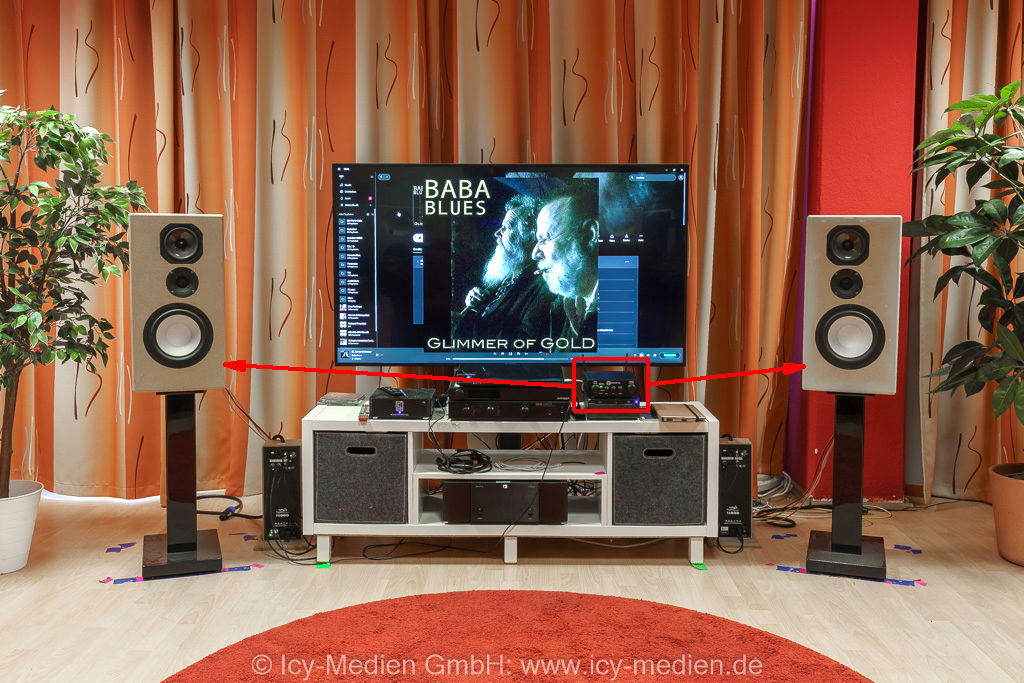
Measurements:
In our article The RTA Module in REW (German only) we have already documented in detail our approach of calibrating speakers at the listening position:
- Measurements are taken at the listening position for the left speaker’s chassis and the right speaker’s chassis individually, as well as for both speakers together (with a 3 dB reduction in excitation); for a 3-way speaker, a total of 9 measurements with moving microphone must be taken
- If the speakers are positioned reasonably symmetrically in the room, the frequency response should be largely the same - at least in the midrange and high-frequency ranges - when measuring the left speaker alone, the right speaker alone, and both speakers together -> in that case, the measurement results for both speakers are used for further analysis
- If the three measurements - left, right, and both speakers - differ too much (which often happens in the bass range with an asymmetrical setup), then one speaker is first roughly adjusted to match the other, then both speakers are measured, and the analysis proceeds using these combined results
- Based on these moving microphone measurements at the listening position and background information on the drivers (directivity, total harmonic distortion, etc.), an acoustic target function is defined for each driver. For 3-way systems, we prefer a Linkwitz-Riley filter slope of 24 dB/octave to ensure that the overlap regions do not become too wide
- At the listening position, we prefer a frequency response that rolls off uniformly at 0.3 dB/terz, 0.9 dB/octave, or 3 dB/decade
- For the moving microphone measurements, the microphone is pointed forward, and the 0° correction curve is used
We would be happy to explain in detail why we take this approach and which physical and psychoacoustic effects are taken into account in one of our activation workshops.
And this is what the measurements look like:
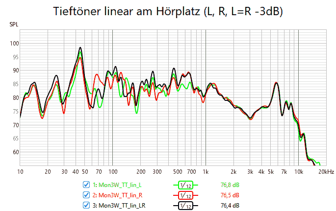
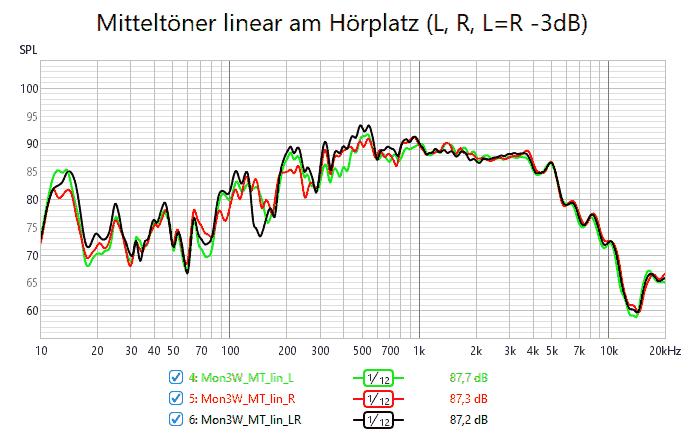
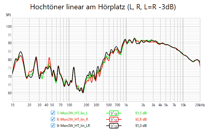
With target crossover frequencies of 400 Hz and 2.5 kHz, the measurements for the tweeter and midrange driver - left (L) only, right (R) only, and both (-3 dB, LR) - align quite well, so we can continue working with the LR curve. In the bass range, there are differences - particularly in the 60 to 150 Hz range - due to the slightly asymmetrical placement in the room; nevertheless, for the sake of simplicity, we will continue working with the LR curve here as well.
Simulation:

Since the measurement results are available in REW, you can now make “virtual” corrections in EQ mode. To do this, it’s best to define an acoustic target function (Target) for each driver (woofer=TT, midrange=MT, tweeter=HT) . . .
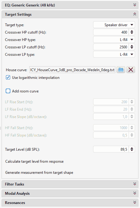
. . . and adjust the settings under EQ Filters until

. . . until the predicted result matches the target function. In doing so, we consider not only the useful frequency range (e.g., 400 Hz to 2.5 kHz for the midrange driver), but also the roll-off slopes down to approximately 20 dB below the useful level. And this is what it looks like for our 3-way monitor speaker:
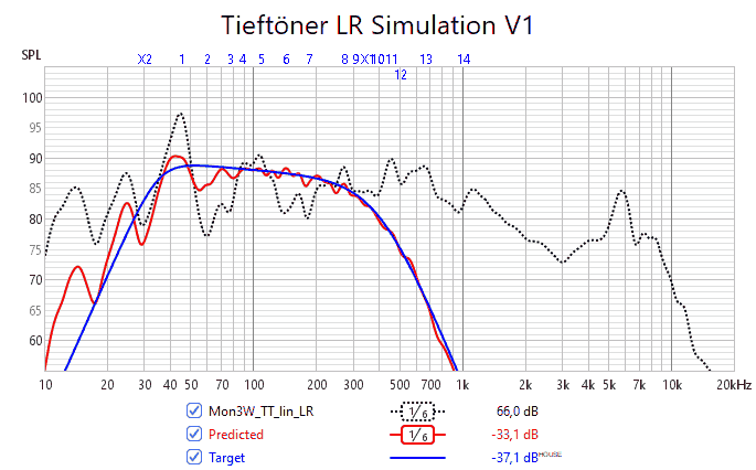
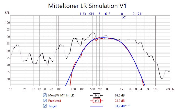
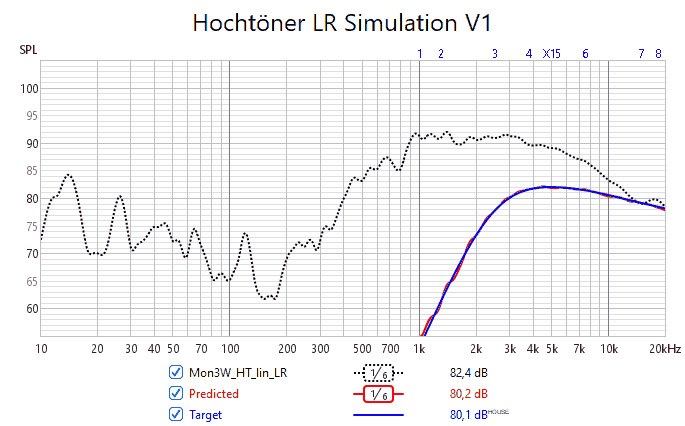
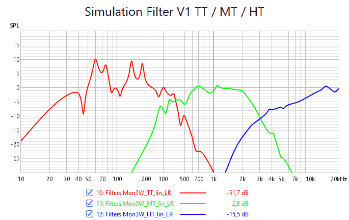
The acoustic target functions were:
| Driver | High-pass | Low-pass | Level |
| Low-frequency | 35 Hz, Butterworth 24 dB/octave | 400 Hz, Linkwitz-Riley 24 dB/octave | 85.0 dB |
| Midrange | 400 Hz, Linkwitz-Riley 24 dB/octave | 2.5 kHz, Linkwitz-Riley 24 dB/octave | 89.5 dB |
| High-frequency | 2.5 kHz, Linkwitz-Riley 24 dB/octave | - | 85.0 dB |
ATTENTION: The different levels of the individual drivers must be achieved through different gain settings in the target device. In the example above, the woofer and tweeter have the same gain; the midrange driver, however, must be attenuated by 4.5 dB, since it was optimized for a target response curve that is 4.5 dB higher!
Transferring the simulation results to the target hardware:
If you are satisfied with the predicted result, you must transfer the found values to the hardware. With many DSP systems (e.g., HYPEX FusionAmp), this requires manual work. You have to constantly switch back and forth between the measurement/simulation software REW and the hardware configuration software, and you must remain highly focused to avoid transfer errors - after all, up to 15 pairs of values for frequency, gain, and Q must be entered and then verified for each branch. In our activation workshops, this is always the point where participants have to take a half-hour coffee break (because I need some peace and quiet while transferring the data) . . . ;-)
It would be much faster and less prone to errors if you could export the values from REW and then import the EQ settings you found into the hardware’s configuration software . . .
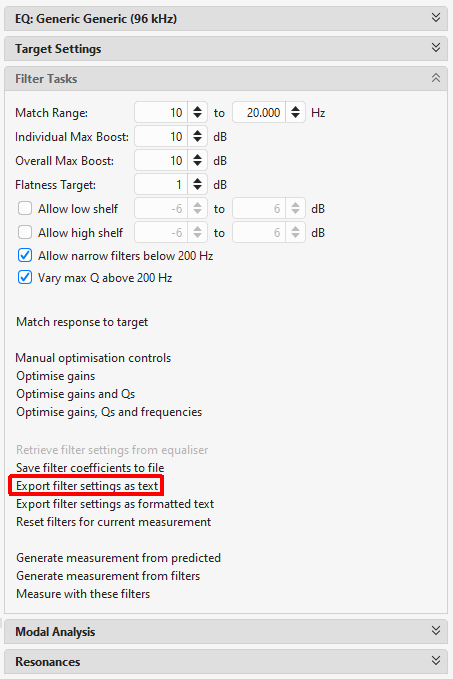
With the combination of AC650DSP and AirDSP, that’s exactly what works! To do this, you first need to save the settings you’ve found in the EQ module as a text file under “Filter task” / “Export filter settings as text.”
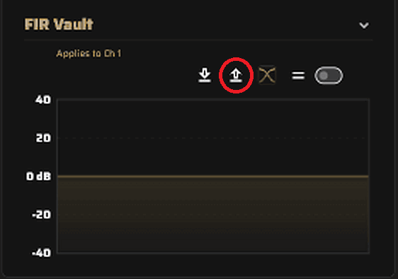
This file can then be imported into the AirDSP software in the 15-band EQ section (4 icons in the upper right corner) - this eliminates the tedious and error-prone manual entry of values (the HYPEX software could take a cue from this) ;-)

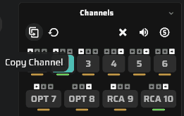
This virtual correction in REW and the subsequent import process into AirDSP must be performed once for each channel. If both speakers are equalized identically, the settings in AirDSP can then be copied from one channel (e.g., left woofer) to the “other” channel (i.e., right woofer) (see below). If the drivers in the left and right speakers have been equalized differently, additional export/import steps are required.
However, the Generic EQ in REW only imports up to 15 EQ settings, NOT the filter settings - you’ll still have to transfer those manually :- (. In a 3-way system, however, that amounts to only 4 values (low-pass for the woofer, high-pass and low-pass for the midrange driver, and high-pass for the tweeter) ;-).
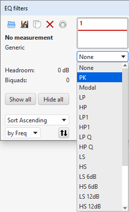
So much for the theory! Before we move on to the practical test, we naturally need to check whether the AC650DSP’s DSP is working “correctly” or “as expected.” Since REW didn’t yet have its own AirDSP EQ at the time of the measurements (it’s available starting with REW V5.40 beta 134), we prefer to use the Generic EQ - this approach is also recommended by ACOUSTAS. However, the Generic EQ has “different” settings:
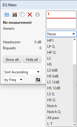
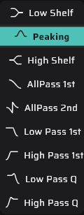
This raises the question:
- What are the names of the settings available in AirDSP in REW?
- and do they behave the same way?
The translation table for the names is still relatively simple:
| AirDSP Name | REW Name | Note |
| Low Shelf | LS Q | |
| Peaking | PK | |
| High Shelf | HS Q | |
| AllPass 1st | Not available in REW | |
| AllPass 2nd | All Pass | |
| Low Pass 1st | LP1 | |
| High Pass 1st | HP1 | |
| Low Pass Q | LP Q | |
| High Pass Q | HP Q |
The crossover frequencies and filter characteristics are entered in the Generic EQ in the X1 and X2 fields. Although these values are exported, AirDSP cannot import them because the import function is limited to the 15-band EQ (in V1.2.14+40).
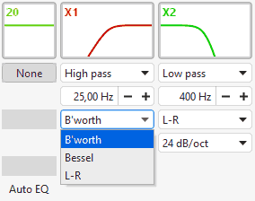
Many of the features available in REW’s Generic EQ are not available in AirDSP - so you must not use these features in REW’s Generic EQ for virtual correction if you want to import the settings found in REW into AirDSP!!! Furthermore, AirDSP provides “only” 15 EQs, whereas the Generic EQ in REW allows for 20 EQs. You must also always ensure that the maximum and minimum input values allowed in AirDSP for frequency, Q, and gain are not exceeded - otherwise, the exported values will not import into AirDSP! In the meantime AirDSP EQ is available in REW (as of REW V5.40 beta 134), so of course you should use that - then you won't have to worry about those "little things" anymore . . .
Transferability of DSP Settings Across Different DSP Systems
When you want to select an EQ in the EQ module in REW, you can’t help but wonder: “Why are there so many? Aren’t they all the same?”
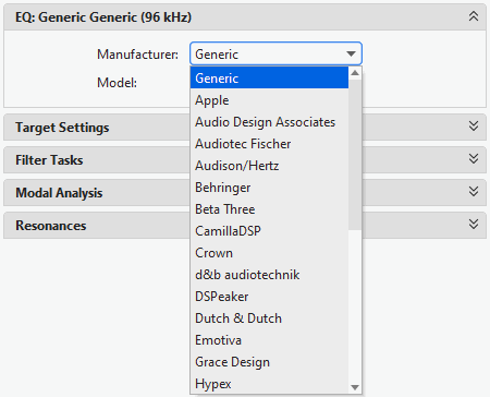
In addition to the differing interpretations of Bessel filters, shelving filters are also interpreted differently across various DSP systems: for example, at the specified frequency, the gain is often not half of the entered gain (midpoint gain) - and as a result, the shelving filter behaves differently than “intended.”
Furthermore, different DSP systems provide varying numbers of EQs with different adjustment ranges and, in some cases, different functions.
And even the seemingly simple PEQ is interpreted differently by various DSP systems: while the gain and frequency may match, there are differing interpretations regarding the Q factor - and as a result, the PEQ behaves differently than “intended” (see below).
Finally, there is the influence of the sampling rate - for example, with PEQs near half the sampling rate (= Nyquist frequency). Here, the measured or simulated frequency response of a PEQ at 16 kHz with a 10 dB boost and a Q factor of 5 is shown at various sampling rates:
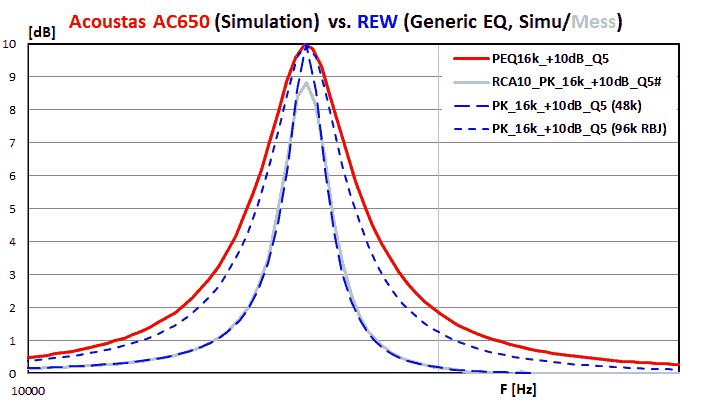
- The measurement (gray) and REW simulation (blue, 48 kHz) match and show a significantly narrower response than at 96 kHz (blue dashed line) or in the ideal case (red)
Note: In version 1.2.14+37, the AC650 simulation still showed the ideal curve (without taking the internal sampling frequency into account);
Starting with version 1.2.14+40, the current internal sampling frequency is taken into account
⇒ Normally, the settings cannot be transferred without further verification!
We compared the frequency responses simulated in AirDSP with those simulated by REW. A very helpful feature came in handy here: in AirDSP, the simulated frequency response can optionally be saved as a CSV file (= Comma Separated Values).
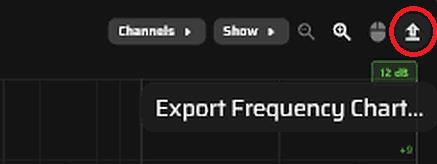
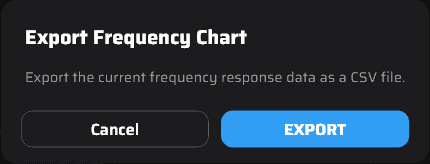
REW also allows you to export measurements - you “just” need to first create a measurement from the simulated filter in the EQ module’s “Filter Tasks” tab (see above) using the “Generate measurement from filter” option ;-)
We worked through the REW/Generic EQ <-> AirDSP conversion table above step by step and found a perfect match for the items listed. In some cases, we didn’t rely solely on the simulations but also measured the response ourselves (see above). This establishes the basis for us to trust that the frequency response predicted in REW will, after applying the filter and EQ settings found in AirDSP or AC650DSP, correspond to the subsequent measurement.
After all, what good is a simulation if the actual measurement turns out differently in the end?!?
Here, then, is the comparison between the simulation in REW (Generic EQ, blue curve), the simulation in AirDSP (red curve), and the measurement (green curve):
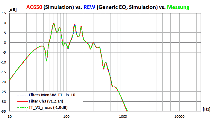
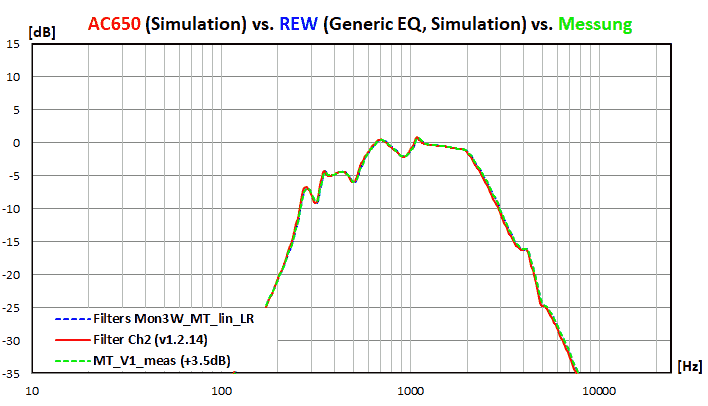
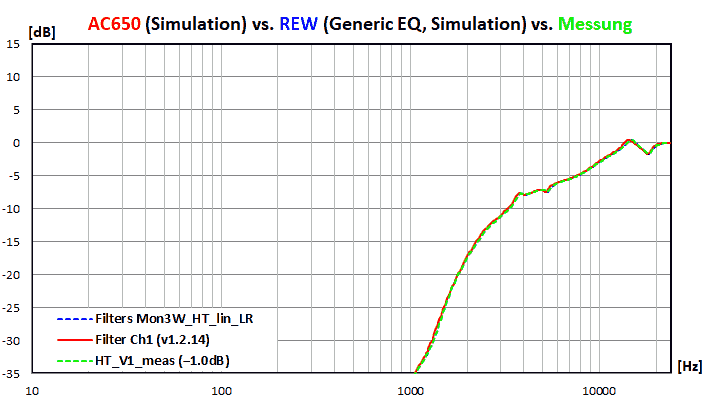
-> All three curves align perfectly; the voltage response on the AC650DSP behaves exactly like the simulation in REW :-)
By the way, this is what the simulation of the frequency response at the listening position would have looked like if the values from the Generic EQ had been applied 1:1 to the HYPEX FusionAmp (left image; on the right, for comparison, the simulation for the AC650DSP from above):
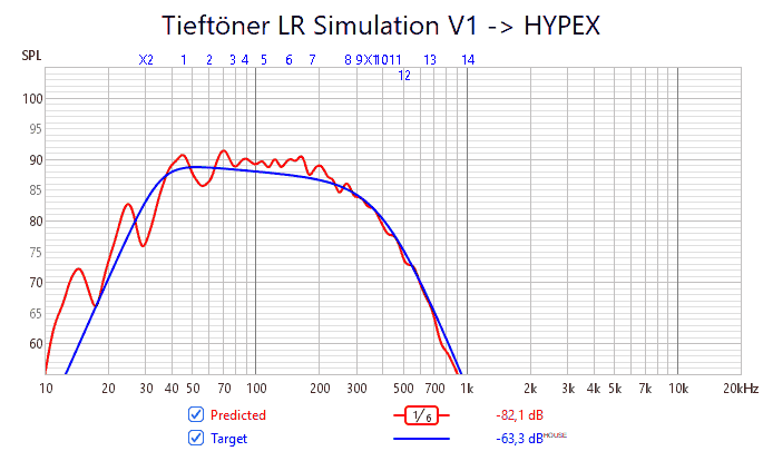
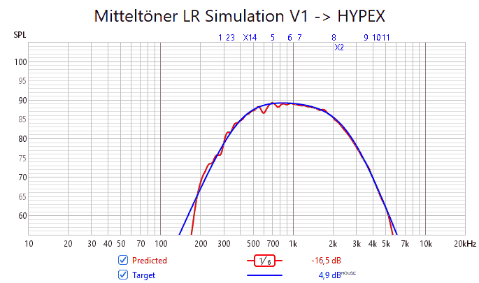
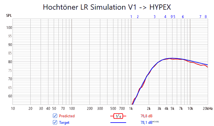
-> Significant differences, particularly in the bass range due to the strong corrections, but also in the high-frequency range (due to the higher sampling frequency)
Measurements at the listening position (V1):
Since the measured voltage response matched the simulation so perfectly, the frequency response at the listening position should also match the simulation. Here is the overall frequency response and the individual channels with both speakers (LR) driven simultaneously:
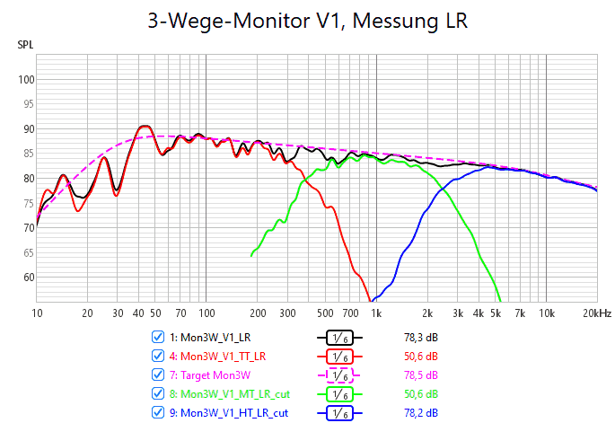
- The overall frequency response (black curve) follows the target curve (magenta) very closely
- the overlap at the crossover frequencies of 400 Hz and 2.5 kHz is good
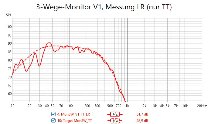
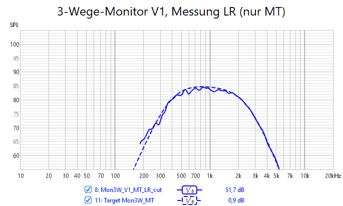
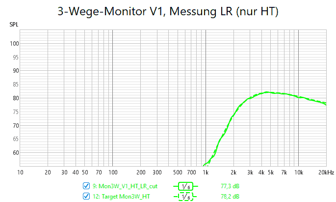
-- the individual branches (low-frequency = TT, mid-frequency = MT, and high-frequency = HT) also follow the target function very closely - just like in the simulation!
Microphone Calibration:It’s great when the measurement curve matches the simulation - but does the measurement curve also match reality? After all, all measurement microphones are more or less prone to error and provide more or less inaccurate readings. Fortunately, there are - of course, individually tailored - correction curves that can be loaded into the measurement software to correct for the specific error of the measurement microphone.But what about the quality of the correction curves? Over the past 20 years, we have calibrated over 4,000 measurement microphones (see 1,000 Microphone Calibrations””An Overview (German only)), some of them multiple times because customers asked us to check their microphones, for example, after they’d been dropped. Of these more than 4,000 microphones, over 700 were miniDSP UMIK-1 models that came with a correction curve provided by the manufacturer. It therefore made sense to examine the deviations between our correction curve and the manufacturer’s correction curve for this model. You can read the results of this analysis in the article Comparison of the Calibration Spectra of the miniDSP UMIK1 (German only) - and they cast a mixed light on the quality of miniDSP’s correction curves . . . |
Determining the Time Delay:
When measuring at the listening position with moving microphone, an energy-based averaging occurs, during which phase information is unfortunately lost. With a Linkwitz-Riley filter, the level at the cutoff frequency has dropped by 6 dB - so a “perfect” summation of the branches is necessary for a linear sum frequency response (note: two signals with equal amplitude result in a only then 6 dB higher sum level if they have the same phase). You can take advantage of this:
- Vary the time delay between the two branches and check whether the sum level increases or decreases
- The time delay that produces the highest sum level is the “correct” time delay, because it ensures that the phases are in phase
We’d be happy to show you the most efficient way to do this in one of our activation workshops.
Here are a few measurement results for the time delay between the midrange (MT) and tweeter (HT) (left: HT delay; right: MT delay):
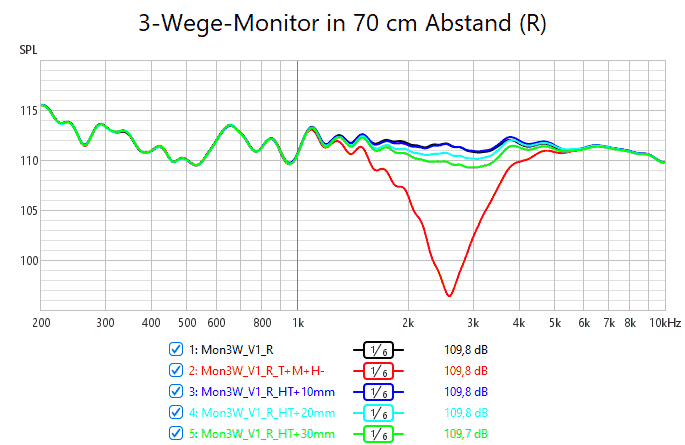
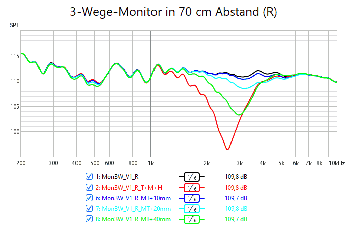
- highest total level at a 0 mm time delay between MT and HT (black curve)
- maximum dip when a driver is reverse-polarized
Even between the woofer and midrange, introducing a time delay did not increase the overall sound level. Thus, the time delay remained at 0 ms for all three channels - thanks to the “lowered” tweeter with waveguide.
Subjective Assessment:
But what good are nice measurement curves if it doesn’t sound good in the end? Well, since the frequency response follows our preferred target curve, the speaker also sounds the way we prefer - at least in terms of tonal balance, because the frequency response alone doesn’t really tell us much more than that. By fine-tuning the time alignment, however, we also know that the timing between the drivers is correct. And through the careful selection of the drivers (e.g., tweeters with waveguides), their arrangement on the baffle (tweeter below midrange driver), and the crossover frequencies, we have also ensured that there are no major dips in the radiation pattern. Together with the acoustic design of our listening room (German only) and the alignment of the speakers toward the listening position, we thus achieve a balanced ratio between direct sound and reflections.
We always use this speaker for our activation workshops, and after activation with the ACOUSTAS AC650DSP, it sounds exactly as we’ve come to expect from other DSP systems - except that the calibration with the AC650DSP and AirDSP duo runs much more “smoothly” than, for example, with the HYPEX FusionAmps! These suffer significantly from the clunky Hypex Frequency Designer (HFD) software, which, for example, doesn’t allow you to import simulation results from REW and requires a complicated conversion of the Q factors for the PEQs (see above). It’s also annoying that you can only “communicate” with one FusionAmp at a time, so you constantly have to plug the USB cable in, out, and into a different module - grrrr.
The only thing we noticed was the somewhat “round” bass - we’re used to a slightly “tighter” bass from the HYPEX FusionAmps. But of course, you can experiment with external power amplifiers connected to the RCA output or, in the bass range, equalize the system channel by channel to match the target curve.
Whether others will like this speaker with this tuning naturally also depends on which target curve you’re optimizing for (see Aspects of Target Curve Design for a DRC System (German only)). Other people may prefer different target curves, possibly depending on their preferred music genre.
But this is exactly where the ACOUSTAS AC650DSP’s tone control really shines: here, you can “gently” adjust the slope of the curve and the balance between bass, midrange, and treble, thereby “crafting” your own target curve without having to change the basic tuning.
Linearization of the phase response:
One possible way to improve the slightly “round” sounding low-frequency range might be to linearize the phase response. This linearization is particularly easy to achieve with AirDSP by selecting the “Linearizer” option in the FIR Builder.
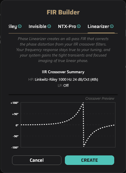
However, you must not correct the currently selected ELECTRICAL filter function there, but rather the ACOUSTIC target function. To do this:
- Temporarily change the electrical cutoff frequencies and filter characteristics to match the acoustic ones (see below),
- Export the FIR coefficients to a text file,
- Import them back immediately,
- and reset the acoustic cutoff frequencies and filter characteristics to the electrical values.
Here is a comparison of the electrical and acoustic filter functions:
| Branch | High-pass filter (electrical) | High-pass filter (acoustic) | Low-pass filter (electrical) | Low-pass filter (acoustic) |
| Low-frequency | Butterworth 12 dB/octave at 30 Hz | Butterworth 36 dB/octave at 35 Hz (Theory) | Butterworth 18 dB/octave at 350 Hz | Linkwitz-Riley 24 dB/octave at 400 Hz |
| Midrange | Butterworth 18 dB/octave at 450 Hz | Linkwitz-Riley 24 dB/octave at 400 Hz | Butterworth 18 dB/octave at 2200 Hz | Linkwitz-Riley 24 dB/octave at 2500 Hz |
| High frequencies | Linkwitz-Riley 12 dB/octave at 4800 Hz | Linkwitz-Riley 24 dB/octave at 2500 Hz | - | - |
And this is what the FIR coefficients (= impulse response) look like:
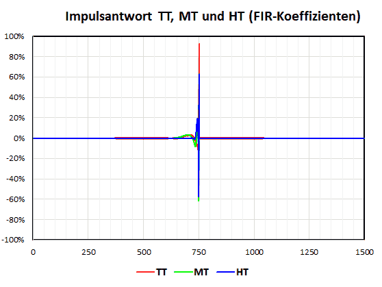
- as you can see, you can’t see a thing!
And this is what they look like when the absolute value of the coefficients is plotted in dB:
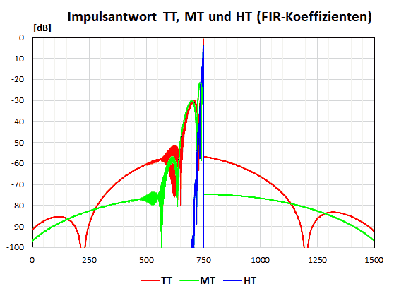
- the FIR coefficients for the tweeter (Linkwitz-Riley high-pass filter with 24 dB/octave at 2.5 kHz) decay quickly
- the FIR coefficients for the woofer and midrange driver have not yet dropped to 0 at the beginning and end
Here you can see that the available 1,500 taps per channel are apparently not sufficient for a filter at 400 Hz. At a sampling rate of 48,000 Hz, 1,500 taps correspond to a frequency resolution of 48,000/1,500 = 32 Hz - and that’s already borderline for accurately reproducing the exact amplitude and phase response. Consequently, this did not work at all for the woofer’s acoustic (high-pass) filter function (Butterworth 36 dB/octave at 35 Hz), so we did not correct for its influence on the acoustic phase response.
The frequency response of a high-pass filter with a Linkwitz-Riley characteristic, a filter slope of 24 dB/octave, and a cutoff frequency of 2.5 kHz (abbreviated: HP2500LR24) looks like this:
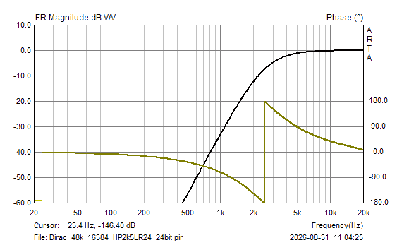
And here is the frequency response of the FIR linearizer’s impulse response for the high-pass filter above:
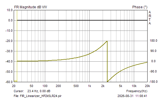
You can see that the impulse response exported using the FIR linearizer does not change the amplitude (0 dB everywhere), but rotates the phase exactly in the opposite direction to the phase of the high-pass filter. This results in a filter that has the desired amplitude response but a phase of 0 everywhere.
So much for the theory. But what does the step response look like with and without the linearizer? At a distance of about 70 cm from the right speaker, it looks like this:
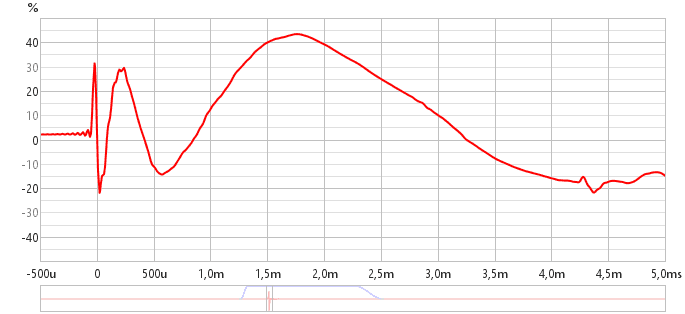
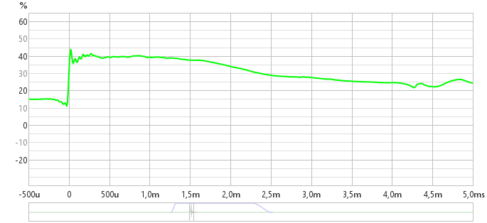
Above (red curve), you can see the typical shape of the step response of a 3-way system:
- first, the narrow peak of the tweeter’s step response
- then, the slightly broader peak of the midrange driver’s step response after about 0.24 ms
- and finally, the broad peak of the woofer’s step response after approximately 1.78 ms
Below (green curve), you can see an almost perfect step response that declines slightly and continuously, since the speaker cannot produce constant sound pressure in the listening room.
Incidentally, this behavior is also visible at the listening position - as the measurements with Dirac Live show. First, the weighted frequency response at the listening position:
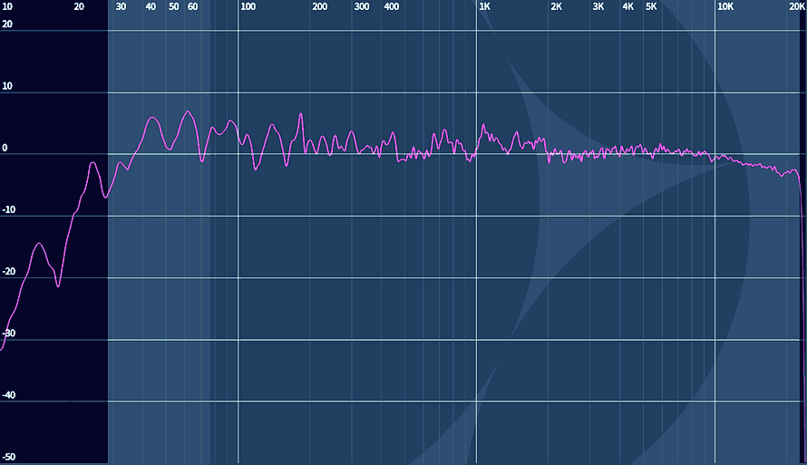
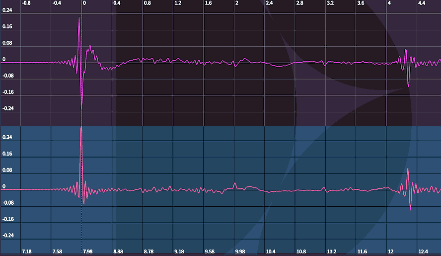
For the impulse responses, the measured impulse response is always shown at the top, while the simulated impulse response with Dirac Live correction is shown at the bottom. First, the impulse responses without the FIR linearizer:
And now with the FIR linearizer:
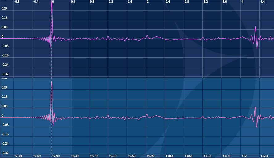
-> When measuring with the FIR linearizer, there’s hardly any noticeable change or improvement from Dirac Live!
And how does it sound with the FIR linearizer? Although the step response looks worlds better, the audible difference is rather subtle. For many tracks, the differences were very minor and didn’t lead to a clear preference for one version over the other. With electronic music, the differences were sometimes more clearly audible (e.g., Franceen Thirteen / Queen Mary), and in these cases, the version with the FIR linearizer was preferred:
- the wandering percussive patterns (e.g., at the beginning) and the “sound of the surf” (starting at 0:57) had finer temporal resolution
- in particular, the first bass beat at 0.25 sounded “faster” and “drier”
When comparing the setup with and without Dirac, it was noticeable that the bass range sounded “cleaner” with Dirac in all situations - here, the frequency response of both the left and right speakers individually, as well as the sum of both speakers, was largely linear. In our setup, we had “only” optimized the sum of the two speakers and accepted minor deviations in the individual speakers - there is obviously still potential here, but it’s nearly impossible to achieve “manually,” since this requires taking both amplitude and phase into account.
In the midrange and high-frequency ranges, Dirac resulted in only minimal changes. The midrange localization was (as usual) slightly more precise, but (as usual) there was a bit less “air” around the instruments.
With the FIR linearizer option, the difference between using Dirac and not using it was even smaller; it came a bit closer to the effect of Dirac Live.
A detailed sound evaluation of the ACOUSTAS AC650DSP when used with its various inputs””both as a pure preamplifier and as an amplifier for a passive speaker””will follow in Part 3 of our article series. There, we’ll also explain which test tracks we use and what subtle details we pay attention to in order to reach our conclusion.
Conclusion:
With the combination of the ACOUSTAS AC650DSP and AirDSP, speaker calibration becomes a breeze:
- For the initial measurements, only an individually calibrated (USB) microphone is needed; sound output occurs directly via the AC650DSP (USB input)
- For each channel (woofer, midrange, and tweeter), the left (L) and right (R) speakers are measured individually, and additionally, both speakers are measured at a level 3 dB lower (LR)
- Next, simulate the effect of the individual filters and EQs in the Generic EQ in REW (or in the AirDSP EQ starting with REW V5.40 beta 134),
- save the result to a text file,
- import it into the EQ section of AirDSP,
- apply the filters used in the simulation, if necessary,
- adjust the levels, if necessary (in case of different target levels),
- and measure the individual channels and the entire system again
Thanks to the perfect synchronization between REW and AirDSP, this can be achieved on the very first run - see our measurements!
The FIR Linearizer is another tool available, if needed, to optimize the system’s step response.
In principle, you can do the same thing with a HYPEX FusionAmp, but:
- you’ll need an additional sound card to play back the excitation signal
- the results from the Generic-EQ cannot be imported directly (the Q-values must be converted, and all values must be entered manually -> risk of data entry errors!)
- Communication with two devices (one individual FusionAmp for the left channel and one for the right) isn’t possible in parallel; instead, you have to constantly switch the USB cable from the PC between the left and right FusionAmps - which is a pain!
- The entire workflow is significantly more “cumbersome” than with the AC650DSP and AirDSP
With the HYPEX FusionAmps as well (starting with firmware version 5.5), you can use the FIR filters to linearize the phase of the individual channels - but the FusionAmps only have a frequency resolution of 93,750/1,500 = 62.5 Hz, and you have to generate the FIR filters manually using, for example, rePhase. You also have to figure out the correct export format in rePhase so that the FIR coefficients can be read by the Hypex Frequency Designer - this is far from a “smooth” workflow . . .
Another advantage of the AC650DSP is that it can equalize a total of 10 channels - making 3-way systems with Double-Bass-Array subwoofers possible. The fact that the built-in amplifiers in the AC650DSP may not provide sufficient power in the bass range could be considered a drawback; however, any amplifier can easily be connected via the additional channels, making the system more flexible and adaptable to any changing (power) requirements.
Overall, the combination of the ACOUSTAS AC650DSP and AirDSP completely won us over - it’s never been easier to set up a multi-way speaker system and achieve an ideal step response! In comparison, calibrating the system with the combination of the HYPEX FusionAmp and the Frequency Designer feels like a chore . . .
Afterword:
When we began testing the ACOUSTAS AC650DSP and AirDSP in August 2026, there was still no AirDSP EQ in REW, and the 1.2.13+37 software version was not yet perfect in some areas (e.g., accounting for the sampling rate when displaying the filter response). But in recent weeks - partly thanks to our suggestions - there have been significant developments in the AirDSP software, and an AirDSP EQ has been available in REW since the end of August. Further changes are planned here (e.g., automatic application of filters X1 and X2 as well), so that you, the user, have as little to worry about as possible.
However, we were still using the Generic EQ in REW and therefore initially had to go through a time-consuming process to verify whether it behaved the same way as the hardware. As a user of the AC650DSP, you no longer need to do that - if you measure with REW and use the AirDSP-EQ. We’ve kept this chapter (Transferability of DSP Settings Across Different DSP Systems) anyway, because some users might be measuring with different software or struggling with other hardware where the simulation using the Generic-EQ doesn’t match the behavior of their hardware. This gives you an idea of which settings “typically” might cause problems . . .
We hope we haven't confused you too much with this “mess” (Generic-EQ instead of AirDSP-EQ, different behavior across different software versions) . . .
